
Learn OpenCV by Examples - with Python

You can access my work in all areas on my website www.bulentsiyah.com
About OpenCV
- Officially launched in 1999, OpenCV (Open Source Computer Vision) from an Intel initiative.
- OpenCV's core is written in C++. In python we are simply using a wrapper that executes C++ code inside of python.
- First major release 1.0 was in 2006, second in 2009, third in 2015 and 4th in 2018. with OpenCV 4.0 Beta.
- It is an Open source library containing over 2500 optimized algorithms.
- It is EXTREMELY useful for almost all computer vision applications and is supported on Windows, Linux, MacOS, Android, iOS with bindings to Python, Java and Matlab.
Update(19.05.2020))
I will always try to improve this kernel. I made some additions to this version. Thanks for reading, I hope it will be useful
Newly Added Content
- 17.Background Subtraction Methods
- 18.Funny Mirrors Using OpenCV
Content
- Sharpening
- Thresholding, Binarization & Adaptive Thresholding
- Dilation, Erosion, Opening and Closing
- Edge Detection & Image Gradients
- Perpsective Transform
- Scaling, re-sizing and interpolations
- Image Pyramids
- Cropping
- Blurring
- Contours
- Approximating Contours and Convex Hull
- Identifiy Contours by Shape
- Line Detection - Using Hough Lines
- Counting Circles and Ellipses
- Finding Corners
- Finding Waldo
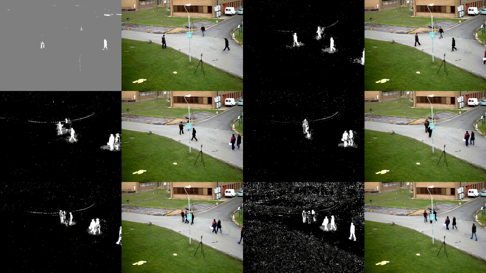
- Background Subtraction Methods
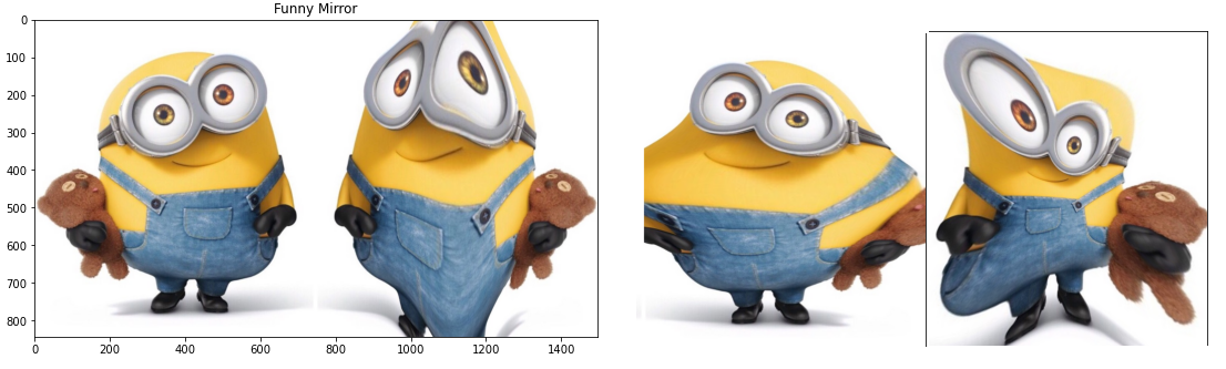
- Funny Mirrors Using OpenCV
Background Subtraction Methods Output
Funny Mirrors Using OpenCV Output
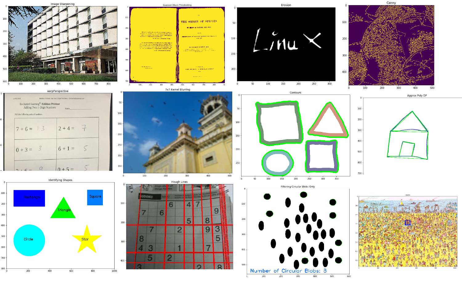
Some pictures from content
In [1]:
import numpy as np import matplotlib.pyplot as plt import cv2
By altering our kernels we can implement sharpening, which has the effects of in strengthening or emphasizing edges in an image.
In [2]:
image = cv2.imread('/kaggle/input/opencv-samples-images/data/building.jpg') image = cv2.cvtColor(image, cv2.COLOR_BGR2RGB) plt.figure(figsize=(20, 20)) plt.subplot(1, 2, 1) plt.title("Original") plt.imshow(image) # Create our shapening kernel, we don't normalize since the # the values in the matrix sum to 1 kernel_sharpening = np.array([[-1,-1,-1], [-1,9,-1], [-1,-1,-1]]) # applying different kernels to the input image sharpened = cv2.filter2D(image, -1, kernel_sharpening) plt.subplot(1, 2, 2) plt.title("Image Sharpening") plt.imshow(sharpened) plt.show()

In [3]:
# Load our new image image = cv2.imread('/kaggle/input/opencv-samples-images/Origin_of_Species.jpg', 0) plt.figure(figsize=(30, 30)) plt.subplot(3, 2, 1) plt.title("Original") plt.imshow(image) # Values below 127 goes to 0 (black, everything above goes to 255 (white) ret,thresh1 = cv2.threshold(image, 127, 255, cv2.THRESH_BINARY) plt.subplot(3, 2, 2) plt.title("Threshold Binary") plt.imshow(thresh1) # It's good practice to blur images as it removes noise image = cv2.GaussianBlur(image, (3, 3), 0) # Using adaptiveThreshold thresh = cv2.adaptiveThreshold(image, 255, cv2.ADAPTIVE_THRESH_MEAN_C, cv2.THRESH_BINARY, 3, 5) plt.subplot(3, 2, 3) plt.title("Adaptive Mean Thresholding") plt.imshow(thresh) _, th2 = cv2.threshold(image, 0, 255, cv2.THRESH_BINARY + cv2.THRESH_OTSU) plt.subplot(3, 2, 4) plt.title("Otsu's Thresholding") plt.imshow(th2) plt.subplot(3, 2, 5) # Otsu's thresholding after Gaussian filtering blur = cv2.GaussianBlur(image, (5,5), 0) _, th3 = cv2.threshold(blur, 0, 255, cv2.THRESH_BINARY + cv2.THRESH_OTSU) plt.title("Guassian Otsu's Thresholding") plt.imshow(th3) plt.show()

In [4]:
image = cv2.imread('/kaggle/input/opencv-samples-images/data/LinuxLogo.jpg') image = cv2.cvtColor(image, cv2.COLOR_BGR2RGB) plt.figure(figsize=(20, 20)) plt.subplot(3, 2, 1) plt.title("Original") plt.imshow(image) # Let's define our kernel size kernel = np.ones((5,5), np.uint8) # Now we erode erosion = cv2.erode(image, kernel, iterations = 1) plt.subplot(3, 2, 2) plt.title("Erosion") plt.imshow(erosion) # dilation = cv2.dilate(image, kernel, iterations = 1) plt.subplot(3, 2, 3) plt.title("Dilation") plt.imshow(dilation) # Opening - Good for removing noise opening = cv2.morphologyEx(image, cv2.MORPH_OPEN, kernel) plt.subplot(3, 2, 4) plt.title("Opening") plt.imshow(opening) # Closing - Good for removing noise closing = cv2.morphologyEx(image, cv2.MORPH_CLOSE, kernel) plt.subplot(3, 2, 5) plt.title("Closing") plt.imshow(closing)
Out[4]:
<matplotlib.image.AxesImage at 0x7fa9340f9f60>

In [5]:
image = cv2.imread('/kaggle/input/opencv-samples-images/data/fruits.jpg') image = cv2.cvtColor(image, cv2.COLOR_BGR2RGB) height, width,_ = image.shape # Extract Sobel Edges sobel_x = cv2.Sobel(image, cv2.CV_64F, 0, 1, ksize=5) sobel_y = cv2.Sobel(image, cv2.CV_64F, 1, 0, ksize=5) plt.figure(figsize=(20, 20)) plt.subplot(3, 2, 1) plt.title("Original") plt.imshow(image) plt.subplot(3, 2, 2) plt.title("Sobel X") plt.imshow(sobel_x) plt.subplot(3, 2, 3) plt.title("Sobel Y") plt.imshow(sobel_y) sobel_OR = cv2.bitwise_or(sobel_x, sobel_y) plt.subplot(3, 2, 4) plt.title("sobel_OR") plt.imshow(sobel_OR) laplacian = cv2.Laplacian(image, cv2.CV_64F) plt.subplot(3, 2, 5) plt.title("Laplacian") plt.imshow(laplacian) ## Then, we need to provide two values: threshold1 and threshold2. Any gradient value larger than threshold2 # is considered to be an edge. Any value below threshold1 is considered not to be an edge. #Values in between threshold1 and threshold2 are either classified as edges or non-edges based on how their #intensities are “connected”. In this case, any gradient values below 60 are considered non-edges #whereas any values above 120 are considered edges. # Canny Edge Detection uses gradient values as thresholds # The first threshold gradient canny = cv2.Canny(image, 50, 120) plt.subplot(3, 2, 6) plt.title("Canny") plt.imshow(canny)
Out[5]:
<matplotlib.image.AxesImage at 0x7fa925f28358>

/opt/conda/lib/python3.6/site-packages/matplotlib/cm.py:273: RuntimeWarning: invalid value encountered in multiply xx = (xx * 255).astype(np.uint8)

In [6]:
image = cv2.imread('/kaggle/input/opencv-samples-images/scan.jpg') image = cv2.cvtColor(image, cv2.COLOR_BGR2RGB) plt.figure(figsize=(20, 20)) plt.subplot(1, 2, 1) plt.title("Original") plt.imshow(image) # Cordinates of the 4 corners of the original image points_A = np.float32([[320,15], [700,215], [85,610], [530,780]]) # Cordinates of the 4 corners of the desired output # We use a ratio of an A4 Paper 1 : 1.41 points_B = np.float32([[0,0], [420,0], [0,594], [420,594]]) # Use the two sets of four points to compute # the Perspective Transformation matrix, M M = cv2.getPerspectiveTransform(points_A, points_B) warped = cv2.warpPerspective(image, M, (420,594)) plt.subplot(1, 2, 2) plt.title("warpPerspective") plt.imshow(warped)
Out[6]:
<matplotlib.image.AxesImage at 0x7fa9374e1908>

Re-sizing is very easy using the cv2.resize function, it's arguments are: cv2.resize(image, dsize(output image size), x scale, y scale, interpolation)
In [7]:
image = cv2.imread('/kaggle/input/opencv-samples-images/data/fruits.jpg') image = cv2.cvtColor(image, cv2.COLOR_BGR2RGB) plt.figure(figsize=(20, 20)) plt.subplot(2, 2, 1) plt.title("Original") plt.imshow(image) # Let's make our image 3/4 of it's original size image_scaled = cv2.resize(image, None, fx=0.75, fy=0.75) plt.subplot(2, 2, 2) plt.title("Scaling - Linear Interpolation") plt.imshow(image_scaled) # Let's double the size of our image img_scaled = cv2.resize(image, None, fx=2, fy=2, interpolation = cv2.INTER_CUBIC) plt.subplot(2, 2, 3) plt.title("Scaling - Cubic Interpolation") plt.imshow(img_scaled) # Let's skew the re-sizing by setting exact dimensions img_scaled = cv2.resize(image, (900, 400), interpolation = cv2.INTER_AREA) plt.subplot(2, 2, 4) plt.title("Scaling - Skewed Size") plt.imshow(img_scaled)
Out[7]:
<matplotlib.image.AxesImage at 0x7fa9374055c0>

Useful when scaling images in object detection.
In [8]:
image = cv2.imread('/kaggle/input/opencv-samples-images/data/butterfly.jpg') image = cv2.cvtColor(image, cv2.COLOR_BGR2RGB) plt.figure(figsize=(20, 20)) plt.subplot(2, 2, 1) plt.title("Original") plt.imshow(image) smaller = cv2.pyrDown(image) larger = cv2.pyrUp(smaller) plt.subplot(2, 2, 2) plt.title("Smaller") plt.imshow(smaller) plt.subplot(2, 2, 3) plt.title("Larger") plt.imshow(larger)
Out[8]:
<matplotlib.image.AxesImage at 0x7fa925e03710>

In [9]:
image = cv2.imread('/kaggle/input/opencv-samples-images/data/messi5.jpg') image = cv2.cvtColor(image, cv2.COLOR_BGR2RGB) plt.figure(figsize=(20, 20)) plt.subplot(2, 2, 1) plt.title("Original") plt.imshow(image) height, width = image.shape[:2] # Let's get the starting pixel coordiantes (top left of cropping rectangle) start_row, start_col = int(height * .25), int(width * .25) # Let's get the ending pixel coordinates (bottom right) end_row, end_col = int(height * .75), int(width * .75) # Simply use indexing to crop out the rectangle we desire cropped = image[start_row:end_row , start_col:end_col] plt.subplot(2, 2, 2) plt.title("Cropped") plt.imshow(cropped)
Out[9]:
<matplotlib.image.AxesImage at 0x7fa925d6c0b8>

In [10]:
image = cv2.imread('/kaggle/input/opencv-samples-images/data/home.jpg') image = cv2.cvtColor(image, cv2.COLOR_BGR2RGB) plt.figure(figsize=(20, 20)) plt.subplot(2, 2, 1) plt.title("Original") plt.imshow(image) # Creating our 3 x 3 kernel kernel_3x3 = np.ones((3, 3), np.float32) / 9 # We use the cv2.fitler2D to conovlve the kernal with an image blurred = cv2.filter2D(image, -1, kernel_3x3) plt.subplot(2, 2, 2) plt.title("3x3 Kernel Blurring") plt.imshow(blurred) # Creating our 7 x 7 kernel kernel_7x7 = np.ones((7, 7), np.float32) / 49 blurred2 = cv2.filter2D(image, -1, kernel_7x7) plt.subplot(2, 2, 3) plt.title("7x7 Kernel Blurring") plt.imshow(blurred2)
Out[10]:
<matplotlib.image.AxesImage at 0x7fa925cab128>

In [11]:
# Let's load a simple image with 3 black squares image = cv2.imread('/kaggle/input/opencv-samples-images/data/pic3.png') image = cv2.cvtColor(image, cv2.COLOR_BGR2RGB) plt.figure(figsize=(20, 20)) plt.subplot(2, 2, 1) plt.title("Original") plt.imshow(image) # Grayscale gray = cv2.cvtColor(image,cv2.COLOR_BGR2GRAY) # Find Canny edges edged = cv2.Canny(gray, 30, 200) plt.subplot(2, 2, 2) plt.title("Canny Edges") plt.imshow(edged) # Finding Contours # Use a copy of your image e.g. edged.copy(), since findContours alters the image contours, hierarchy = cv2.findContours(edged, cv2.RETR_EXTERNAL, cv2.CHAIN_APPROX_NONE) plt.subplot(2, 2, 3) plt.title("Canny Edges After Contouring") plt.imshow(edged) print("Number of Contours found = " + str(len(contours))) # Draw all contours # Use '-1' as the 3rd parameter to draw all cv2.drawContours(image, contours, -1, (0,255,0), 3) plt.subplot(2, 2, 4) plt.title("Contours") plt.imshow(image)

Number of Contours found = 4
Out[11]:
<matplotlib.image.AxesImage at 0x7fa925b185c0>

cv2.approxPolyDP(contour, Approximation Accuracy, Closed)
- contour -- is the individual contour we wish to approximate
- Approximation Accuracy -- Important parameter is determining the accuracy of the approximation. Small values give precise- approximations, large values give more generic approximation. A good rule of thumb is less than 5% of the contour perimeter
- Closed -- a Boolean value that states whether the approximate contour should be open or closed
In [12]:
# Load image and keep a copy image = cv2.imread('/kaggle/input/opencv-samples-images/house.jpg') image = cv2.cvtColor(image, cv2.COLOR_BGR2RGB) plt.figure(figsize=(20, 20)) plt.subplot(2, 2, 1) plt.title("Original") plt.imshow(image) orig_image = image.copy() # Grayscale and binarize gray = cv2.cvtColor(image, cv2.COLOR_BGR2GRAY) ret, thresh = cv2.threshold(gray, 127, 255, cv2.THRESH_BINARY_INV) # Find contours contours, hierarchy = cv2.findContours(thresh.copy(), cv2.RETR_LIST, cv2.CHAIN_APPROX_NONE) # Iterate through each contour and compute the bounding rectangle for c in contours: x,y,w,h = cv2.boundingRect(c) cv2.rectangle(orig_image,(x,y),(x+w,y+h),(0,0,255),2) plt.subplot(2, 2, 2) plt.title("Bounding Rectangle") plt.imshow(orig_image) cv2.waitKey(0) # Iterate through each contour and compute the approx contour for c in contours: # Calculate accuracy as a percent of the contour perimeter accuracy = 0.03 * cv2.arcLength(c, True) approx = cv2.approxPolyDP(c, accuracy, True) cv2.drawContours(image, [approx], 0, (0, 255, 0), 2) plt.subplot(2, 2, 3) plt.title("Approx Poly DP") plt.imshow(image) plt.show() # Convex Hull image = cv2.imread('/kaggle/input/opencv-samples-images/hand.jpg') gray = cv2.cvtColor(image, cv2.COLOR_BGR2GRAY) plt.figure(figsize=(20, 20)) plt.subplot(1, 2, 1) plt.title("Original Image") plt.imshow(image) # Threshold the image ret, thresh = cv2.threshold(gray, 176, 255, 0) # Find contours contours, hierarchy = cv2.findContours(thresh.copy(), cv2.RETR_LIST, cv2.CHAIN_APPROX_NONE) # Sort Contors by area and then remove the largest frame contour n = len(contours) - 1 contours = sorted(contours, key=cv2.contourArea, reverse=False)[:n] # Iterate through contours and draw the convex hull for c in contours: hull = cv2.convexHull(c) cv2.drawContours(image, [hull], 0, (0, 255, 0), 2) plt.subplot(1, 2, 2) plt.title("Convex Hull") plt.imshow(image)

/opt/conda/lib/python3.6/site-packages/matplotlib/figure.py:98: MatplotlibDeprecationWarning: Adding an axes using the same arguments as a previous axes currently reuses the earlier instance. In a future version, a new instance will always be created and returned. Meanwhile, this warning can be suppressed, and the future behavior ensured, by passing a unique label to each axes instance. "Adding an axes using the same arguments as a previous axes "


In [13]:
image = cv2.imread('/kaggle/input/opencv-samples-images/someshapes.jpg') image = cv2.cvtColor(image, cv2.COLOR_BGR2RGB) gray = cv2.cvtColor(image, cv2.COLOR_BGR2GRAY) plt.figure(figsize=(20, 20)) plt.subplot(2, 2, 1) plt.title("Original") plt.imshow(image) ret, thresh = cv2.threshold(gray, 127, 255, 1) # Extract Contours contours, hierarchy = cv2.findContours(thresh.copy(), cv2.RETR_LIST, cv2.CHAIN_APPROX_NONE) for cnt in contours: # Get approximate polygons approx = cv2.approxPolyDP(cnt, 0.01*cv2.arcLength(cnt,True),True) if len(approx) == 3: shape_name = "Triangle" cv2.drawContours(image,[cnt],0,(0,255,0),-1) # Find contour center to place text at the center M = cv2.moments(cnt) cx = int(M['m10'] / M['m00']) cy = int(M['m01'] / M['m00']) cv2.putText(image, shape_name, (cx-50, cy), cv2.FONT_HERSHEY_SIMPLEX, 1, (0, 0, 0), 2) elif len(approx) == 4: x,y,w,h = cv2.boundingRect(cnt) M = cv2.moments(cnt) cx = int(M['m10'] / M['m00']) cy = int(M['m01'] / M['m00']) # Check to see if 4-side polygon is square or rectangle # cv2.boundingRect returns the top left and then width and if abs(w-h) <= 3: shape_name = "Square" # Find contour center to place text at the center cv2.drawContours(image, [cnt], 0, (0, 125 ,255), -1) cv2.putText(image, shape_name, (cx-50, cy), cv2.FONT_HERSHEY_SIMPLEX, 1, (0, 0, 0), 2) else: shape_name = "Rectangle" # Find contour center to place text at the center cv2.drawContours(image, [cnt], 0, (0, 0, 255), -1) M = cv2.moments(cnt) cx = int(M['m10'] / M['m00']) cy = int(M['m01'] / M['m00']) cv2.putText(image, shape_name, (cx-50, cy), cv2.FONT_HERSHEY_SIMPLEX, 1, (0, 0, 0), 2) elif len(approx) == 10: shape_name = "Star" cv2.drawContours(image, [cnt], 0, (255, 255, 0), -1) M = cv2.moments(cnt) cx = int(M['m10'] / M['m00']) cy = int(M['m01'] / M['m00']) cv2.putText(image, shape_name, (cx-50, cy), cv2.FONT_HERSHEY_SIMPLEX, 1, (0, 0, 0), 2) elif len(approx) >= 15: shape_name = "Circle" cv2.drawContours(image, [cnt], 0, (0, 255, 255), -1) M = cv2.moments(cnt) cx = int(M['m10'] / M['m00']) cy = int(M['m01'] / M['m00']) cv2.putText(image, shape_name, (cx-50, cy), cv2.FONT_HERSHEY_SIMPLEX, 1, (0, 0, 0), 2) plt.subplot(2, 2, 2) plt.title("Identifying Shapes") plt.imshow(image)
Out[13]:
<matplotlib.image.AxesImage at 0x7fa9257c8470>

cv2.HoughLines(binarized/thresholded image, 𝜌 accuracy, 𝜃 accuracy, threshold)
- Threshold here is the minimum vote for it to be considered a line
In [14]:
image = cv2.imread('/kaggle/input/opencv-samples-images/data/sudoku.png') image = cv2.cvtColor(image, cv2.COLOR_BGR2RGB) plt.figure(figsize=(20, 20)) # Grayscale and Canny Edges extracted gray = cv2.cvtColor(image, cv2.COLOR_BGR2GRAY) edges = cv2.Canny(gray, 100, 170, apertureSize = 3) plt.subplot(2, 2, 1) plt.title("edges") plt.imshow(edges) # Run HoughLines using a rho accuracy of 1 pixel # theta accuracy of np.pi / 180 which is 1 degree # Our line threshold is set to 240 (number of points on line) lines = cv2.HoughLines(edges, 1, np.pi/180, 200) # We iterate through each line and convert it to the format # required by cv.lines (i.e. requiring end points) for line in lines: rho, theta = line[0] a = np.cos(theta) b = np.sin(theta) x0 = a * rho y0 = b * rho x1 = int(x0 + 1000 * (-b)) y1 = int(y0 + 1000 * (a)) x2 = int(x0 - 1000 * (-b)) y2 = int(y0 - 1000 * (a)) cv2.line(image, (x1, y1), (x2, y2), (255, 0, 0), 2) plt.subplot(2, 2, 2) plt.title("Hough Lines") plt.imshow(image)
Out[14]:
<matplotlib.image.AxesImage at 0x7fa925768860>

In [15]:
image = cv2.imread('/kaggle/input/opencv-samples-images/blobs.jpg') image = cv2.cvtColor(image, cv2.COLOR_BGR2RGB) plt.figure(figsize=(20, 20)) # Intialize the detector using the default parameters detector = cv2.SimpleBlobDetector_create() # Detect blobs keypoints = detector.detect(image) # Draw blobs on our image as red circles blank = np.zeros((1,1)) blobs = cv2.drawKeypoints(image, keypoints, blank, (0,0,255), cv2.DRAW_MATCHES_FLAGS_DRAW_RICH_KEYPOINTS) number_of_blobs = len(keypoints) text = "Total Number of Blobs: " + str(len(keypoints)) cv2.putText(blobs, text, (20, 550), cv2.FONT_HERSHEY_SIMPLEX, 1, (100, 0, 255), 2) # Display image with blob keypoints plt.subplot(2, 2, 1) plt.title("Blobs using default parameters") plt.imshow(blobs) # Set our filtering parameters # Initialize parameter settiing using cv2.SimpleBlobDetector params = cv2.SimpleBlobDetector_Params() # Set Area filtering parameters params.filterByArea = True params.minArea = 100 # Set Circularity filtering parameters params.filterByCircularity = True params.minCircularity = 0.9 # Set Convexity filtering parameters params.filterByConvexity = False params.minConvexity = 0.2 # Set inertia filtering parameters params.filterByInertia = True params.minInertiaRatio = 0.01 # Create a detector with the parameters detector = cv2.SimpleBlobDetector_create(params) # Detect blobs keypoints = detector.detect(image) # Draw blobs on our image as red circles blank = np.zeros((1,1)) blobs = cv2.drawKeypoints(image, keypoints, blank, (0,255,0), cv2.DRAW_MATCHES_FLAGS_DRAW_RICH_KEYPOINTS) number_of_blobs = len(keypoints) text = "Number of Circular Blobs: " + str(len(keypoints)) cv2.putText(blobs, text, (20, 550), cv2.FONT_HERSHEY_SIMPLEX, 1, (0, 100, 255), 2) # Show blobs plt.subplot(2, 2, 2) plt.title("Filtering Circular Blobs Only") plt.imshow(blobs)
Out[15]:
<matplotlib.image.AxesImage at 0x7fa92569a6d8>

In [16]:
# Load image then grayscale image = cv2.imread('/kaggle/input/opencv-samples-images/data/chessboard.png') image = cv2.cvtColor(image, cv2.COLOR_BGR2RGB) plt.figure(figsize=(10, 10)) gray = cv2.cvtColor(image, cv2.COLOR_BGR2GRAY) # The cornerHarris function requires the array datatype to be float32 gray = np.float32(gray) harris_corners = cv2.cornerHarris(gray, 3, 3, 0.05) #We use dilation of the corner points to enlarge them\ kernel = np.ones((7,7),np.uint8) harris_corners = cv2.dilate(harris_corners, kernel, iterations = 10) # Threshold for an optimal value, it may vary depending on the image. image[harris_corners > 0.025 * harris_corners.max() ] = [255, 127, 127] plt.subplot(1, 1, 1) plt.title("Harris Corners") plt.imshow(image)
Out[16]:
<matplotlib.image.AxesImage at 0x7fa925618dd8>

In [17]:
# Load input image and convert to grayscale image = cv2.imread('/kaggle/input/opencv-samples-images/WaldoBeach.jpg') image = cv2.cvtColor(image, cv2.COLOR_BGR2RGB) plt.figure(figsize=(30, 30)) plt.subplot(2, 2, 1) plt.title("Where is Waldo?") plt.imshow(image) gray = cv2.cvtColor(image, cv2.COLOR_BGR2GRAY) # Load Template image template = cv2.imread('/kaggle/input/opencv-samples-images/waldo.jpg',0) result = cv2.matchTemplate(gray, template, cv2.TM_CCOEFF) min_val, max_val, min_loc, max_loc = cv2.minMaxLoc(result) #Create Bounding Box top_left = max_loc bottom_right = (top_left[0] + 50, top_left[1] + 50) cv2.rectangle(image, top_left, bottom_right, (0,0,255), 5) plt.subplot(2, 2, 2) plt.title("Waldo") plt.imshow(image)
Out[17]:
<matplotlib.image.AxesImage at 0x7fa9255abc88>

source: https://docs.opencv.org/3.4/d1/dc5/tutorial_background_subtraction.html
How to Use Background Subtraction Methods
Background subtraction (BS) is a common and widely used technique for generating a foreground mask (namely, a binary image containing the pixels belonging to moving objects in the scene) by using static cameras.
As the name suggests, BS calculates the foreground mask performing a subtraction between the current frame and a background model, containing the static part of the scene or, more in general, everything that can be considered as background given the characteristics of the observed scene.

In [18]:
import cv2 import matplotlib.pyplot as plt algo = 'MOG2' if algo == 'MOG2': backSub = cv2.createBackgroundSubtractorMOG2() else: backSub = cv2.createBackgroundSubtractorKNN() plt.figure(figsize=(20, 20)) frame = cv2.imread('/kaggle/input/opencv-samples-images/Background_Subtraction_Tutorial_frame.png') fgMask = backSub.apply(frame) plt.subplot(2, 2, 1) plt.title("Frame") plt.imshow(cv2.cvtColor(frame, cv2.COLOR_BGR2RGB)) plt.subplot(2, 2, 2) plt.title("FG Mask") plt.imshow(cv2.cvtColor(fgMask, cv2.COLOR_BGR2RGB)) frame = cv2.imread('/kaggle/input/opencv-samples-images/Background_Subtraction_Tutorial_frame_1.png') fgMask = backSub.apply(frame) plt.subplot(2, 2, 3) plt.title("Frame") plt.imshow(cv2.cvtColor(frame, cv2.COLOR_BGR2RGB)) plt.subplot(2, 2, 4) plt.title("FG Mask") plt.imshow(cv2.cvtColor(fgMask, cv2.COLOR_BGR2RGB))
Out[18]:
<matplotlib.image.AxesImage at 0x7fa9254bea20>

If you want to run it on video and locally, you must set it to (While) True. (Do not try on Kaggle you will get the error)-True.-(Do-not-try-on-Kaggle-you-will-get-the-error))
In [19]:
import cv2 import numpy as np algo = 'MOG2' inputt = '/kaggle/input/opencv-samples-images/video_input/Background_Subtraction_Tutorial_frame.mp4' capture = cv2.VideoCapture(cv2.samples.findFileOrKeep(inputt)) frame_width = int(capture.get(3)) frame_height = int(capture.get(4)) out = cv2.VideoWriter('Background_Subtraction_Tutorial_frame_output.mp4',cv2.VideoWriter_fourcc('M','J','P','G'),30, (frame_width,frame_height)) if algo == 'MOG2': backSub = cv2.createBackgroundSubtractorMOG2() else: backSub = cv2.createBackgroundSubtractorKNN() # If you want to run it on video and locally, you must set it to (While) True. (Do not try on Kaggle you will get the error) while False: ret, frame = capture.read() if frame is None: break fgMask = backSub.apply(frame) cv2.rectangle(frame, (10, 2), (100,20), (255,255,255), -1) cv2.imshow('Frame', frame) cv2.imshow('FG Mask', fgMask) out.write(cv2.cvtColor(fgMask, cv2.COLOR_BGR2RGB)) keyboard = cv2.waitKey(1) & 0xFF; if (keyboard == 27 or keyboard == ord('q')): cv2.destroyAllWindows() break; capture.release() out.release() cv2.destroyAllWindows()
The result you will get on video and locally
Source: https://www.learnopencv.com/funny-mirrors-using-opencv/
Funny mirrors are not plane mirrors but a combination of convex/concave reflective surfaces that produce distortion effects that look funny as we move in front of these mirrors.
How does it work ?
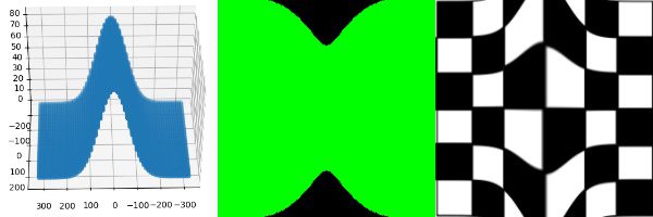
The entire project can be divided into three major steps :
- Create a virtual camera.
- Define a 3D surface (the mirror surface) and project it into the virtual camera using a suitable value of projection matrix.
- Use the image coordinates of the projected points of the 3D surface to apply mesh based warping to get the desired effect of a funny mirror.
In [20]:
!pip install vcam

Collecting vcam Downloading https://files.pythonhosted.org/packages/5a/81/31e561c9e2be275df47e313786932ce8e176f29616b65c19a1ef23ccaa3b/vcam-1.0-py3-none-any.whl Installing collected packages: vcam Successfully installed vcam-1.0
In [21]:
import cv2 import numpy as np import math from vcam import vcam,meshGen import matplotlib.pyplot as plt plt.figure(figsize=(20, 20)) # Reading the input image. Pass the path of image you would like to use as input image. img = cv2.imread("/kaggle/input/opencv-samples-images/minions.jpg") H,W = img.shape[:2] # Creating the virtual camera object c1 = vcam(H=H,W=W) # Creating the surface object plane = meshGen(H,W) # We generate a mirror where for each 3D point, its Z coordinate is defined as Z = 20*exp^((x/w)^2 / 2*0.1*sqrt(2*pi)) plane.Z += 20*np.exp(-0.5*((plane.X*1.0/plane.W)/0.1)**2)/(0.1*np.sqrt(2*np.pi)) pts3d = plane.getPlane() pts2d = c1.project(pts3d) map_x,map_y = c1.getMaps(pts2d) output = cv2.remap(img,map_x,map_y,interpolation=cv2.INTER_LINEAR) plt.subplot(1, 2,1) plt.title("Funny Mirror") plt.imshow(cv2.cvtColor(np.hstack((img,output)), cv2.COLOR_BGR2RGB))
Out[21]:
<matplotlib.image.AxesImage at 0x7fa9259626a0>

So now as we know that by defining Z as a function of X and Y we can create different types of distortion effects. Let us create some more effects using the above code. We simply need to change the line where we define Z as a function of X and Y. This will further help you to create your own effects.
In [22]:
plt.figure(figsize=(20, 20)) # Reading the input image. Pass the path of image you would like to use as input image. img = cv2.imread("/kaggle/input/opencv-samples-images/minions.jpg") H,W = img.shape[:2] # Creating the virtual camera object c1 = vcam(H=H,W=W) # Creating the surface object plane = meshGen(H,W) # We generate a mirror where for each 3D point, its Z coordinate is defined as Z = 20*exp^((y/h)^2 / 2*0.1*sqrt(2*pi)) plane.Z += 20*np.exp(-0.5*((plane.Y*1.0/plane.H)/0.1)**2)/(0.1*np.sqrt(2*np.pi)) pts3d = plane.getPlane() pts2d = c1.project(pts3d) map_x,map_y = c1.getMaps(pts2d) output = cv2.remap(img,map_x,map_y,interpolation=cv2.INTER_LINEAR) plt.subplot(1, 2,1) plt.title("Funny Mirror") plt.imshow(cv2.cvtColor(np.hstack((img,output)), cv2.COLOR_BGR2RGB))
Out[22]:
<matplotlib.image.AxesImage at 0x7fa9258bbdd8>

Let's create something using sine function !
In [23]:
plt.figure(figsize=(20, 20)) # Reading the input image. Pass the path of image you would like to use as input image. img = cv2.imread("/kaggle/input/opencv-samples-images/minions.jpg") H,W = img.shape[:2] # Creating the virtual camera object c1 = vcam(H=H,W=W) # Creating the surface object plane = meshGen(H,W) # We generate a mirror where for each 3D point, its Z coordinate is defined as Z = 20*[ sin(2*pi*(x/w-1/4))) + sin(2*pi*(y/h-1/4))) ] plane.Z += 20*np.sin(2*np.pi*((plane.X-plane.W/4.0)/plane.W)) + 20*np.sin(2*np.pi*((plane.Y-plane.H/4.0)/plane.H)) pts3d = plane.getPlane() pts2d = c1.project(pts3d) map_x,map_y = c1.getMaps(pts2d) output = cv2.remap(img,map_x,map_y,interpolation=cv2.INTER_LINEAR) plt.subplot(1, 2,1) plt.title("Funny Mirror") plt.imshow(cv2.cvtColor(np.hstack((img,output)), cv2.COLOR_BGR2RGB))
Out[23]:
<matplotlib.image.AxesImage at 0x7fa925a115f8>


